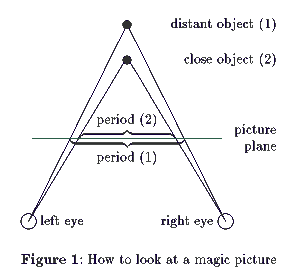
The new technique differs from the conventional way to present stereographic views: Instead of having two independent views of the same scene, taken from slightly different angles, all the data here are contained in one picture, which must be looked at with a squint, so the visual axes cross behind (or in front of) the picture, and intersect the picture plane at a certain distance.

Seeing how much has been written about it, I wont give here a detailed description of the phenomenon. Suffice it to say that the secret of the 3D effect is that the graphical information on the picture is roughly periodic, the period being the distance of the section points of the visual axes with the picture plane. If the periodicity is perfect, the whole picture is seen as flat. Everywhere the periodicity is disturbed details stand out in relief, seeming closer if the periodicity is less and more distant if it is greater (cf. figure 1).
For input, we describe a picture as a two-dimensional grid of numbers, each number meaning the height of the point it denotes. The number 0 stands for the lowest (most distant) plane. Only numbers between 0 and 9 are allowed. A semicolon delimits a line. The data shown in figure 2 describe a small rectangle that floats one unit above the ground plane.
000000000000000000000000000000;
000000000000000000000000000000;
000000000000000000000000000000;
000000000000111111000000000000;
000000000000111111000000000000;
000000000000111111000000000000;
000000000000111111000000000000;
000000000000111111000000000000;
000000000000111111000000000000;
000000000000000000000000000000;
000000000000000000000000000000;
000000000000000000000000000000;
Figure 2: Input data for a very simple picture
While it would be possible to construct patterns from black and white dots and to draw them, e. g., as \vrules, this process is very slow and consumes a lot of TeX's resources. Unless the pictures are to show very fine details, it is easier to use patterns built from normal TeX glyphs, such as letters and figures. To facilitate the calculation of the period length, we use a mono-spacing font, \tt.
Each picture element is produced by a call of the \Pixel macro. Its only argument denotes the altitude of the point. According to this argument, the pattern (contained in \Pat) is shifted around and the correct glyph \A for the new element is printed:
  1 \newcount\alt
  2 \def\Pixel#1{
  3    \def\Head##1##2!{##1}
  4    \def\Tail##1##2!{##2}
  5    \edef\A{\expandafter\Head\Pat!}
  6    \edef\Rest{\expandafter\Tail\Pat!}
  7    \edef\T{\Rest}
  8    \alt=#1
  9    \loop\ifnum\alt>0
 10        \edef\A{\expandafter\Head\T!}
 11        \edef\T{\expandafter\Tail\T!}
 12        \advance\alt -1
 13    \repeat
 14    \edef\Pat{\Rest\A}
 15    \A
 16 }
To produce a line of pixels, this macro must be iterated until a semicolon is reached. This is done by the following macro, \Line, which calls itself recursively until it sees a semicolon:
 17 \def\Line#1{
 18     \if #1;\vskip 0pt \else
 19         \Pixel#1
 20         \expandafter\Line
 21     \fi
 22 }
We now could simply give an initial value for \verb_\Pat_ and bracket each line of the picture data by \Line ... ;. The pattern, however, loses details each time it is shifted to a shorter period, and cannot recover the lost information when periods become longer again. We could end up with a pattern consisting of one sort of glyphs only. So it is better to restore a reasonable value at the beginning of each line. This is done in the following macro, \DLine; we simply use the same start pattern for all lines.
 23 \def\DLine#1;{
 24     \edef\Pat{\StartPattern}
 25     \Line#1;
 26 }
Now let's have a look at the result of the following calls, shown in figure 2:
 27 \edef\StartPattern{A-CeL+MX-/()pd=}
 28 \DLine 000000000000000000000000000000;
... (as in figure 1)
The effect of figure 3 is not very convincing as the picture is simply too small: it does not even show two full periods of the pattern. Now we could inflate the data to make the picture larger; on the other hand, TeX can do this for us. We just have to change the following lines in our macro definitions:
19 \Pixel#1\Pixel#1\Pixel#1
25 \Line#1;\Line#1;
to blow up each pixel to a 3 x 2 matrix. (To do this with loops is left as an exercise to the reader.) The above data (trimmed somewhat to fit into the column) then yield the picture in figure 4.
Now, if you have a trained magic eye, you should be able to see the floating rectangle in the middle of figure 4, and a somewhat more informative picture in figure 5. (If you have no experience with such pictures, ask somebody who has, or simply try staring at it, or forget about the whole thing--its not really vital after all!) Figure 5 shows that it can be useful to compress the picture vertically, by specifying a negative \vskip in line 18.
Possible extensions of the macros presented are: